Dy(III) complex: the point-dipole approximation#

This tutorial works through the main SimpNMR workflows on a dysprosium(III) complex, using the point-dipole approximation for the hyperfine coupling.

For a lanthanide such as Dy(III), the unpaired electrons occupy core-like 4f orbitals that are well shielded from the ligands. The electron–nucleus hyperfine interaction is then dominated by the through-space dipolar coupling, which depends only on the position of each nucleus relative to the paramagnetic centre. SimpNMR computes this directly from the molecular geometry (hyperfine: method: pdip) — no quantum-chemistry hyperfine calculation is required. (For transition-metal complexes, where covalent delocalisation makes the Fermi-contact term important, hyperfine tensors are instead read from a DFT calculation; see Fe(II) complex: DFT-calculated hyperfine tensors.)

The tutorial covers three workflows on the same complex:

Prerequisites#

Install simpnmr by following the Installation guide (which covers pip as well as the double-click Windows and macOS apps), then check it is available:

simpnmr --version

Command line or the desktop app#

Every workflow below can be run either from the terminal (the simpnmr command) or from the desktop GUI. Each step shows both — pick whichever tab you prefer.

The GUI presents the same options as a form and can open and save the very run.yml files shown in this tutorial. To use it, install the optional GUI dependencies and launch it:

pip install "simpnmr[gui]"
simpnmr-gui

The window has a toolbar (New, Open YAML…, Save YAML, Save As…, ▶ Run, ■ Stop); a scrollable form on the left whose sections mirror the run.yml blocks (Hyperfine, Nuclei, Diamagnetic, Susceptibility, …) with a Workflow selector at the top (Predict / Fit susceptibility); and a 3D structure viewer with a live log panel on the right. The general pattern is always the same: Open YAML… → choose your run.yml (the form fills in) → set the Workflow mode → click ▶ Run; output streams in the log panel and files are written to the project folder.

The complex and its input files#

Create a working directory with the data/ sub-folders that will hold the input files:

mkdir dy-tutorial
cd dy-tutorial
mkdir -p data/hfc data/labels data/dia

The workflows below share three input files: the molecular structure, the chemical-label map, and the diamagnetic reference shifts. The magnetic susceptibility is not supplied as a file here — in the first workflow it is generated from a crystal-field parameter, and in the last it is fitted. Create each file with a plain-text editor, copying the contents exactly (use the copy button in the top-right of each block).

The molecular structure — an XYZ file: the first line is the atom count, the second is a comment (blank here), and each remaining line is an element symbol followed by its Cartesian coordinates in Å:

The chemical-label map — assigns each hydrogen atom to a chemical group so that symmetry-equivalent nuclei are averaged together:

The diamagnetic reference shifts — measured on an isostructural diamagnetic analogue, one value per chemical group (ppm):

data/dia/diamagnetic_shifts.csv#

chem_label,shift,
ceq,2.87,
cax,3.67,
ceqp,2.66,
caxp,2.27,
aax,4.15,
aeq,4.08,
py3,8.09,
py4,8.19,
py5,7.75,

1. Predicting the paramagnetic shifts#

The standard prediction workflow computes paramagnetic ¹H shifts from the structure and a susceptibility tensor. Here the susceptibility is not read from a file but generated from a single crystal-field parameter, the second-rank axial Stevens parameter B²₀ (set to −100 cm⁻¹), using Bleaney theory. Create the configuration file run.yml next to the data/ folder:

run.yml#

project:
  name: dy_prediction

hyperfine:
  method: pdip
  file: data/hfc/structure.xyz
  paramagnetic_centre: Dy1
  spin: 2.5
  orbit: 5
  total_momentum_J: 7.5

nuclei:
  include: H

diamagnetic:
  method: csv
  file: data/dia/diamagnetic_shifts.csv

chem_labels:
  file: data/labels/chemical_labels.csv

susceptibility:
  method: bleaney
  bleaney:
    B20: -100.0
    B22: 0.0
    alpha: 0.0
    beta: 0.0
    gamma: 0.0
  temperatures: 302.15

The blocks have the following roles:

project: Names the run. All outputs are written to a directory with this name (here, dy_prediction/). Choose something descriptive for your own system.
hyperfine: method: pdip computes point-dipole hyperfine tensors directly from the structure. The paramagnetic centre is given as an atom label, Dy1, which is resolved to its coordinates from structure.xyz (you could instead give explicit [x, y, z] coordinates). The Dy(III) quantum numbers are those of the free-ion ⁶H_15/2 ground term: spin = 5/2, orbit = 5, and total_momentum_J = 15/2.
nuclei: Selects which nuclei to predict — here all ¹H nuclei.
diamagnetic: Supplies the diamagnetic reference shifts added to the paramagnetic contributions.
chem_labels: Maps individual atom labels to chemical groups so equivalent nuclei are averaged.
susceptibility: method: bleaney builds the susceptibility tensor from the second-rank crystal-field parameters using Bleaney theory, instead of reading it from a file. B²₀ (here −100 cm⁻¹) is the crystal-field parameter in front of the axial second-rank Stevens operator, B²₂ the rhombic parameter, and α/β/γ the orientation of the crystal-field frame; the isotropic Landé g_J is derived from the Dy(III) quantum numbers above. These crystal-field parameters can be estimated, for example, from the emission spectrum of an isostructural Eu(III) complex. temperatures gives the temperature(s) at which shifts are evaluated.

Note

The YAML input is strict: unknown keys are rejected. See Input YAML Files for the full reference of configuration blocks.

Run the prediction:

Command line

From inside dy-tutorial/:

simpnmr predict run.yml

simpnmr logs each step and finishes with Job finished successfully.

Desktop app

Launch the app: simpnmr-gui.
Click Open YAML… and select the run.yml you created — the form fills in from it.
In the Workflow box at the top, make sure Predict is selected.
Click ▶ Run. Each step is logged in the panel on the right, ending with Job finished successfully; the loaded structure is shown in the 3D viewer.

All results are written to the dy_prediction/ directory:

dy_prediction/
├── peak_data_302.15_K.csv               # per-group averaged shift components
├── hyperfines_and_shifts_302.15_K.csv   # per-atom hyperfines and shift terms
├── susceptibility_tensor.csv            # susceptibility tensor used
├── shift_vs_intensity_302.15_K.csv      # simulated spectrum data
├── pcs_isosurf_302.15_K.cube            # PCS isosurface (cube file)
├── pred_spectrum_302.15_K.pdf           # predicted spectrum
├── pred_shift_spread_302.15_K.pdf       # shift spread per chemical group
├── pred_mean_components_302.15_K.pdf    # shift decomposition per group
├── structure.xyz                        # structure with atom labels
└── chemcraft_structure.xyz              # structure for ChemCraft

Because there is no relaxation block, no relaxation model is applied: there are no R₁/linewidth relaxation-decomposition plots, and the predicted peaks are given a small cosmetic display width (a fixed fraction of the shift range) purely so the spectrum is drawable. Add a relaxation block (workflow 2) to compute physical linewidths and relaxation rates.

The two most useful files are peak_data_302.15_K.csv (one row per chemical group, with the total shift and its diamagnetic / pseudocontact / Fermi-contact decomposition, plus the cosmetic linewidth_avg_auto display width; physical linewidths and R₁/R₂ rates appear only with a relaxation block, as in workflow 2) and hyperfines_and_shifts_302.15_K.csv (one row per nucleus, before averaging). The run also writes pcs_isosurf_302.15_K.cube — an isosurface of the pseudocontact-shift field that can be opened in molecular-visualisation software to display the field around the complex. For a full description of every output file, see Output files.

The predicted spectrum gives a quick visual check of the result:

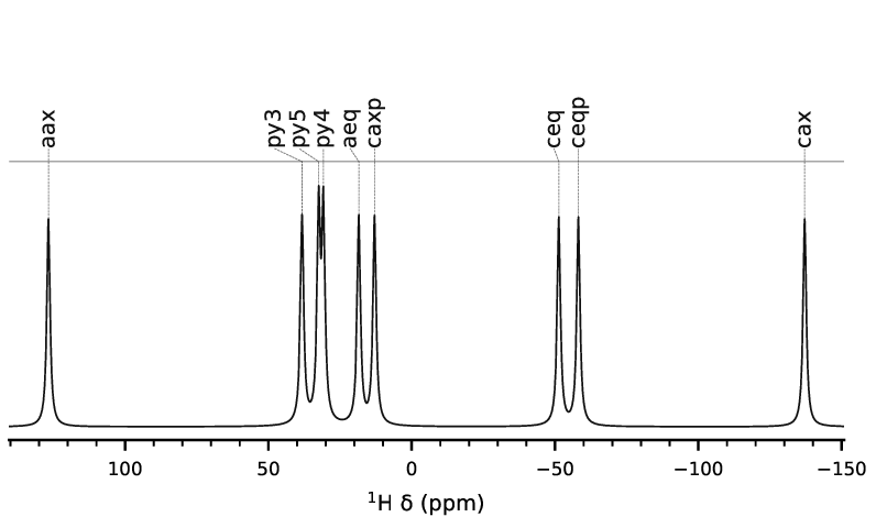
Predicted 1H NMR spectrum of the Dy(III) complex — `pred_spectrum_302.15_K.pdf` — the predicted ¹H spectrum. Each chemical group appears at its averaged paramagnetic shift, spanning roughly +130 to −140 ppm. Because no relaxation model is set, the peaks carry the cosmetic display width described above.#

2. Adding a relaxation model#

Prediction can be extended with a relaxation model to produce predicted linewidths and R₁/R₂ rates alongside the shifts — computed entirely from theory, with no experimental data required. It uses the same shared input files as workflow 1; you add only a relaxation block, giving the electronic and rotational correlation times together with the field and temperature the rates apply to:

run.yml#

project:
  name: dy_prediction_relaxation

hyperfine:
  method: pdip
  file: data/hfc/structure.xyz
  paramagnetic_centre: Dy1
  spin: 2.5
  orbit: 5
  total_momentum_J: 7.5

nuclei:
  include: H

diamagnetic:
  method: csv
  file: data/dia/diamagnetic_shifts.csv

chem_labels:
  file: data/labels/chemical_labels.csv

susceptibility:
  method: bleaney
  bleaney:
    B20: -100.0
    B22: 0.0
    alpha: 0.0
    beta: 0.0
    gamma: 0.0
  temperatures: 302.15

relaxation:
  model: sbm curie
  temperature: 302.15
  magnetic_field_tesla: 4.7
  T1e: 0.2e-12
  T2e: 0.2e-12
  tR: 140.0e-12

The relaxation block adds the transverse (linewidth) and longitudinal (R₁) rates and their SBM-dipolar / contact / Curie decomposition, including the pred_r1_decomposition and pred_linewidth_decomposition plots that were absent in workflow 1.

Then run:

Command line

simpnmr predict run.yml

Desktop app

Launch simpnmr-gui, Open YAML… this run.yml, keep the Workflow on Predict, and click ▶ Run. The relaxation block is picked up automatically, so the run also produces the linewidth and relaxation-rate outputs.

With the relaxation model the predicted peaks now carry physical linewidths:

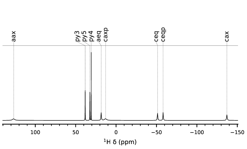
Predicted 1H NMR spectrum of the Dy(III) complex with relaxation — `pred_spectrum_302.15_K.pdf` with the relaxation model. Compare with workflow 1: the peaks farthest from the diamagnetic region (`aax` at +130 ppm, `cax` at −140 ppm) are strongly broadened and shortened by Curie/R₂ relaxation, while the peaks near the centre stay sharp — the position-dependent linewidths the cosmetic display width could not show.#

3. Assignment of experimental peaks and fitting of the magnetic susceptibility#

The inverse of a prediction: rather than computing shifts, we start from a measured ¹H spectrum, assign its paramagnetic peaks to chemical groups, and fit the susceptibility tensor that best reproduces them.

The starting point is the measured spectrum:

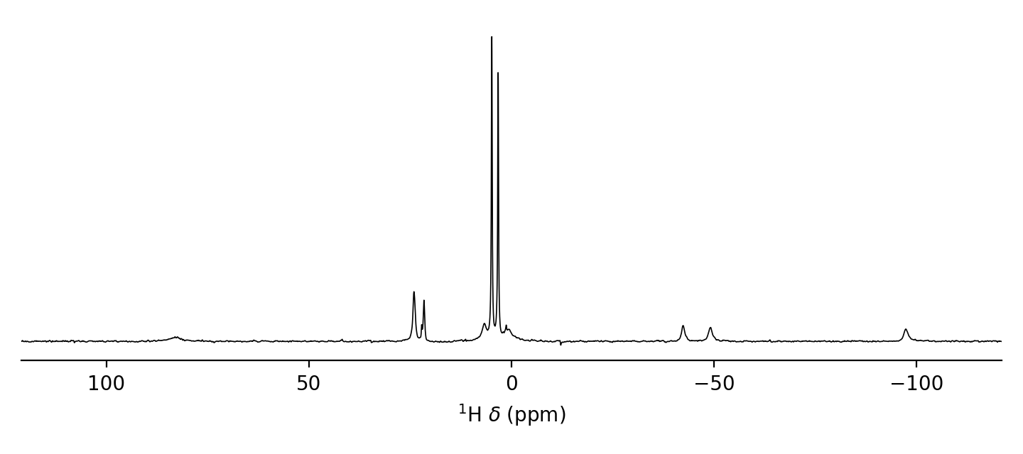
Experimental 1H NMR spectrum of the Dy(III) complex — The measured ¹H spectrum of the complex (`raw_spectrum.csv`), recorded at 302.15 K (29 °C) and 200 MHz (¹H, 4.7 T) in methanol. Sharp peaks near 0 ppm are the diamagnetic region; the well-resolved peaks spread to high and low frequency are the paramagnetically shifted protons that the fit assigns and reproduces.#

Download the spectrum and save it as data/para/raw_spectrum.csv:

raw_spectrum.csv

The spectrum is then deconvoluted — in MestReNova or similar NMR software — into a sum of Lorentzian lineshapes. Each Lorentzian yields a chemical shift, a linewidth, and an integral (area). In addition, the longitudinal relaxation rate R₁ can be measured separately (for example by an inversion–recovery experiment) and included.

These per-peak values make up the experiment.csv — one row per assigned signal, here recorded at 302.15 K and 4.7 T for ¹H:

assignment	shift (ppm)	width (Hz)	area	R₁ (Hz)
`aax`	82.89	587.31	4108.48	—
`py5`	24.14	97.24	5139.3	126
`py3`	23.91	102.86	3914.16	126
`py4`	21.6	74.05	4609	59
`aeq`	6.73	221.6	6320.07	425
`caxp`	0.56	587.4	4984.95	—
`ceqp`	-42.36	182.53	4452.48	400
`ceq`	-49.12	224.78	4826.13	430
`cax`	-97.33	252.06	4772.37	528

where each column is:

assignment — the chemical-group label the peak belongs to (matching the chem_labels map).
shift (ppm) — the measured chemical shift.
width (Hz) — the peak linewidth (full width at half maximum).
area — the integrated peak area.
R₁ (Hz) — the longitudinal relaxation rate (optional; leave the field empty for any peak whose R₁ was not measured, as for aax and caxp here).

Create this as data/para/experiment.csv (run mkdir -p data/para first). The file is plain CSV, with the temperature, field and isotope given as comment lines at the top:

The fit replaces the susceptibility block with an assignment block (which resolves ambiguous peak assignments) and a susc_fit block (which defines the fitted tensor model), and adds an experiment block pointing at the measured data. It reuses the same structure.xyz, chemical_labels.csv and diamagnetic_shifts.csv as workflows 1 and 2.

run.yml#

project:
  name: dy_susceptibility_fit

hyperfine:
  method: pdip
  file: data/hfc/structure.xyz
  paramagnetic_centre: Dy1
  spin: 2.5
  orbit: 5
  total_momentum_J: 7.5

nuclei:
  include: H

assignment:
  method: permute
  groups:
    - [py3, py4, py5]
    - [ceq, ceqp]

diamagnetic:
  method: csv
  file: data/dia/diamagnetic_shifts.csv

experiment:
  files: data/para/experiment.csv
  spectrum_files: data/para/raw_spectrum.csv
  exp_reference: 21.6

chem_labels:
  file: data/labels/chemical_labels.csv

susc_fit:
  type: isoaxrh
  variables:
    iso: [fix, 0.00]
    ax: [fit, 0.001]
    rh_over_ax: [fix, 0.00]
    alpha: [fix, 0.0]
    beta: [fix, 0.0]
    gamma: [fix, 0.0]
  average_shifts: 'all'

The assignment block lists groups of signals whose labelling is ambiguous: the permutation search fits every assignment within each group and keeps the one with the lowest RMSE between the experimental and calculated shifts. Here it tests the three closely spaced pyridine protons py3/py4/py5 (24.14, 23.91 and 21.6 ppm) and the ceq/ceqp pair (−42.36 and −49.12 ppm), whose ordering is not obvious from the spectrum alone. Well-separated signals need not be listed — their assignment is unambiguous.

Run the fit:

Command line

simpnmr fit_susc run.yml

Desktop app

Launch simpnmr-gui, Open YAML… this run.yml, then in the Workflow box switch to Fit susceptibility (this reveals the Assignment and fit-option sections). Click ▶ Run to fit the tensor; the fitted shifts and susceptibility appear in the dy_susceptibility_fit/ folder.

The fit reports the result as a correlation of experimental against calculated shifts, together with the fitted susceptibility and its equivalent crystal-field parameter:

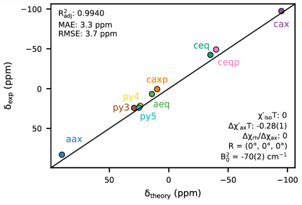
Experimental versus calculated shifts from the susceptibility fit — `shifts_302.15_K.pdf` — experimental against calculated ¹H shifts. The fitted axiality Δχ_ax·T = −0.28(1) corresponds to a Bleaney parameter B²₀ = −70(2) cm⁻¹ (compare the −100 cm⁻¹ used to *generate* the susceptibility in workflow 1) — confirming that this `isoaxrh` fit is the Bleaney fit expressed as susceptibility components. R²_adj = 0.994, RMSE = 3.7 ppm.#

It also overlays the spectrum reconstructed from the fit on the measured one:

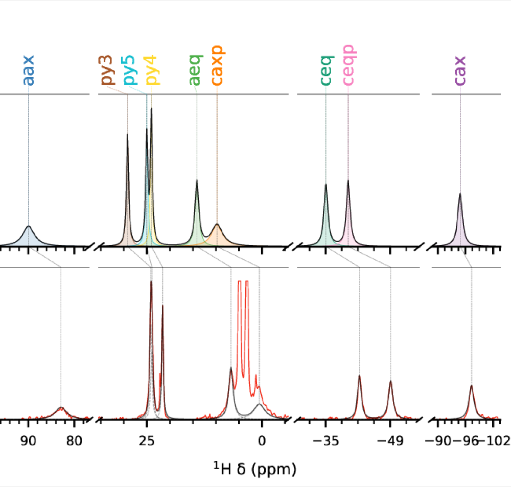
Predicted versus experimental spectrum comparison — `pred_and_exp_spectrum_302.15_K.pdf` — the spectrum reconstructed from the fitted shifts (top, coloured by chemical group) above the measured spectrum (bottom; experiment in black, fit in red), on a broken axis so every paramagnetic peak is visible.#

Next steps#

See Fe(II) complex: DFT-calculated hyperfine tensors for the transition-metal workflow, where hyperfine tensors come from a DFT calculation instead of the point-dipole model.
Read Workflows for an overview of all workflows.
Consult Input YAML Files when adapting run.yml to your own system.